Methodology – How does LandScape+ work?
Landscape model
LandScape+® uses a Python workflow that looks for clusters (groups) of spatial data with similar properties and gives each cluster a unique colour (here referred to as landscape types). The source data used for the models is summarised in Table 1. You can find the specific version of source data for your model in the readme.txt file in your Data Package.
The machine learning does not take any information on the geographical location or soil geochemistry into account. The spatial data layers that are used to cluster the landscape types are selected for their relationship to regolith features and provide information on landscape position, depth of transported cover, and parent and/or regolith materials. To minimise the introduction of human interpretation, LandScape+® does not include surface geology or regolith maps.
| Spatial input layer | Landscape information | Description | Spatial resolution |
|---|---|---|---|
| DEM | General landscape position | Copernicus GLO-30 Digital Elevation Model | ~30 m |
| MrVBF | Estimate of depth of transported cover | Multi-resolution Valley Bottom Flatness index (Gallant et al. 2012) | ~30 m |
| Radiometric data | Indication of parent material | Radiometric data, K pct, U ppm, Th ppm (Poudjom Djomani & Minty 2019) | ~90 m |
| Regolith ratios | Regolith material | A product derived from ratios of bands from Sentinel-2 satellite data (adapted from Gozzard 20051) | ~20 m |
Table 1: Source data layers
The workflow extracts pixel values from spatial data layers for each model area and uses an algorithm, Uniform Manifold Approximation and Projection (UMAP) to reduce each sample point to three dimensions and applies an RGB (red, green, blue) colour scheme. This is referred to as dimensionality reduction. This provides a basis for visualisation and prepares the data for clustering (colouring by groups). An agglomerative hierarchical clustering algorithm is applied to the data with varying numbers of clusters (4 to 16) to separate out different landscape types.
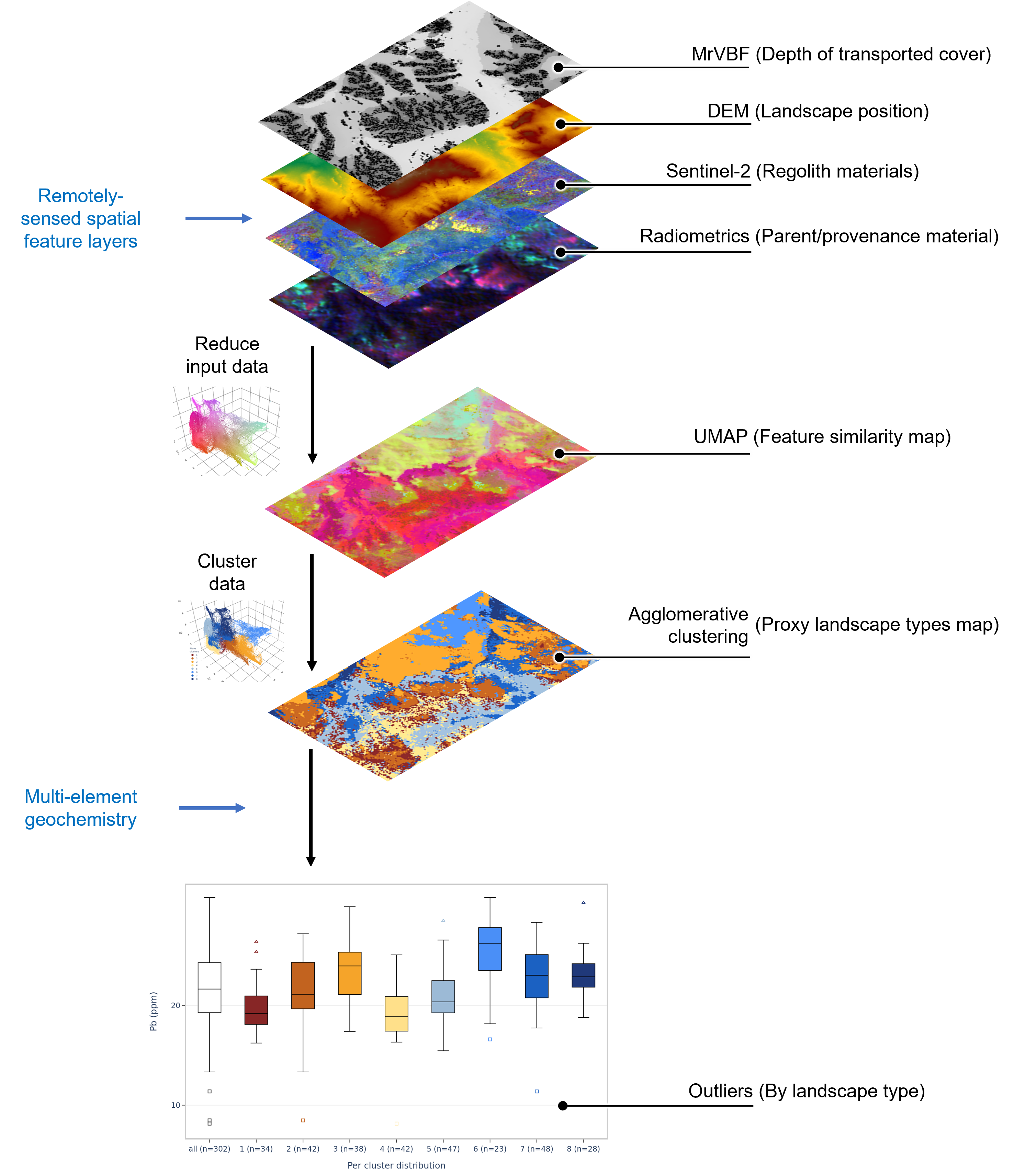
Figure 1: General workflow modified after Henne et al. 2023.
After the data is clustered, each pixel is reassigned its coordinates and projected onto a map coloured by the landscape cluster it belongs to. This is the basis of the clustering model. A 2D map of the pixels coloured by UMAP RGB value is also provided. Ideally the landscape clusters will resemble the UMAP RGB closely.
For a detailed description of the methods, please refer to the open access publications Henne et al. (2023) and (2025).
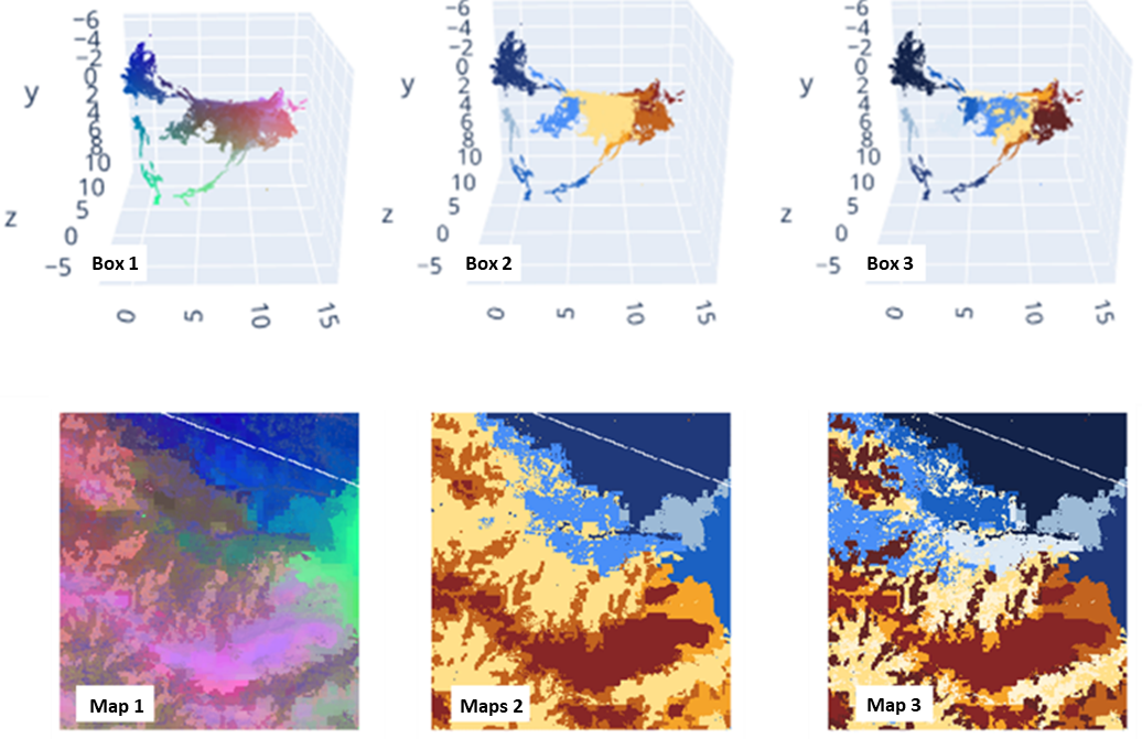
Figure 2: Top row: Examples of clusterboxes showing how pixels are associated in 3D space using an RGB colour scheme (UMAP, Box 1) and coloured by landscape type (Box 2 with eight landscape types, Box 3 with twelve landscape types). Bottom row: Pixels from the clusterboxes projected in 2D spatial context, creating proxy regolith maps with an RGB colour scheme applied (Map1) and with eight (Map 2) and twelve (Map 3) landscape types. The white diagonal line is a masked-out road and is not part of the clustering schemes.
Outlier calculations
Outliers are calculated for each element from the dataset uploaded into LandScape+. Elemental outliers are calculated on log-transformed data and are defined as values that are greater than 1.5 times the interquartile range. Geochemical data are also grouped by their corresponding landscape type and outliers are calculated for each of these landscape types. LandScape+ outputs these as boxplots (Tukey plots) for each element by landscape type and as GeoPackage, ESRI Shapefiles and CSV files.
Principal Component Analysis
The LandScape+ Data Package includes Principal Component Analysis. Principal Component Analysis does not consider landscape types for the results, only the chemistry of the entire survey in the modelled area. Your data must have more elements than principal components (>5). Principal components cannot be viewed in the online User Interface. They can only be accessed in the Data Package download. For more information refer to the Principal Component Analysis section at the end of this document.
-
Gozzard, J.R., 2005. Part 3: Regolith-landform mapping using remotely sensed imagery in IGES 2005. Workshop 1.3, Regolith mapping, workshop notes: Perth, Western Australia, IGES 2005, 73p. ↩