Step 2 - Configure landscape model area
You can define your model area with or without geochemical samples. Samples can also be added, changed or removed later. You can define the model area by
- uploading your sample locations,
- uploading a shape file (e.g., a tenement boundary polygon), or
- drawing a box on a map in the user interface.
Model areas can be configured (or created) in the Add model area tab of your Primary task stepper.
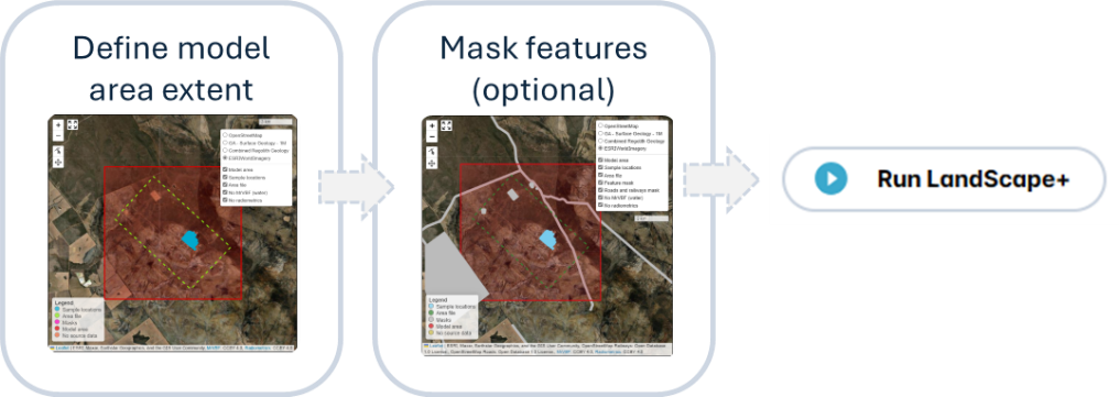
There are three main steps:
- Define the model area extent (using samples, or area file or draw-your-own)_
- (Optional) Mask out features to be excluded from the model area
- Run LandScape+ model (create model)
The software saves your progress when you click on Action buttons (e.g., the Create model button). – If you (or your internet connection) get interrupted, it will pick up near where you left next time you log in.
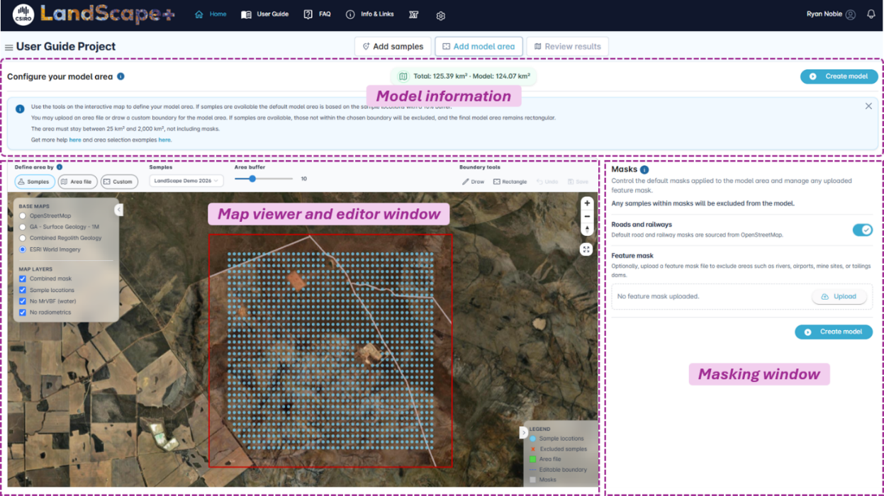
User Interface – Add model area
The Add model area interface contains three areas:
- Model information window
- Map viewer and editor window
- Masking window
Information
The top of the page will prompt you to follow the process for a first-time user. You can return to the previous steps at any time until you run the model. Your settings will only be locked in once you hit “Create model” AND confirm the information message that will pop up. Note, any option from a previous step will still be available to you.
Click on the blue Information button next to “Configure your model area” to expand the help text. You can close this window using the cross in the top right corner.
The Model area calculator (top middle) shows the calculated model area in km². This is automatically updated when you change the extent of the model area or add/remove a mask. This calculated area does not include areas of missing source data or masks. It will remain green if the area is within the enforced bounds (25 km² to 2000 km²) and will turn red if it is too small or too large.
Configuration warnings appear next to the Model area calculator. Clicking this button will provide more information. Commonly this may indicate that samples are outside of the selected model area and will not be included in the analyses.
The Create model button is on the right-hand side of this window and will turn from grey to blue once a valid model area has been created.
Map viewer and editor window
The Map viewer window displays spatial data and is interactive (the model area can be edited within this window). It contains Editing tools above the map, a Legend in the bottom right corner of the map, and a Spatial data toggle for base maps in the top left corner of the map. All toggles can be minimised to give a larger map view if required.
Tools
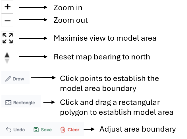
The following tools are available:
Legend
Indicates the colour of different elements.
| Legend item | Description |
|---|---|
| Sample locations | The uploaded samples will display as blue dots if they are in the model area or red crosses if they are outside of the proposed model or fall within a mask (e.g., on a road) |
| Area file (optional) | Area files (e.g., tenement boundary) you upload will display as a shape with a green boundary. Area files are optional and will be uploaded by the user. |
| Masks (optional) | All masks (areas that are excluded from the model, either in-built roads and rails and/or the additional file you upload) will be displayed as grey lines and/or polygons. |
| Model area | The model area will always be a square polygon around either your samples or your area file and will be outlined with a red border. The polygon will turn semi-transparent blue with white point vertices when in edit mode. If in edit mode, the boundary will be dashed. Already existing models will be displayed in semi-transparent purple with a dashed purple outline. |
| No source data | Areas where radiometric measurements and/or MrVBF are not available are displayed as yellow polygons. Both source data are needed to run the model, and such areas will be excluded. MrVBF is not available for permanent waterbodies (as per the source SRTM DEM data at the time of generation). |
Spatial data toggles
The Spatial data toggle allows you to toggle between 4 background layers in the top menu using radio buttons. Only one layer can be displayed at a time.
| Background layers | Description |
|---|---|
| OpenStreetMap | Roads and railways sourced from OpenStreetMap |
| GA – Surface Geology – 1M | Surface Geology of Australia at a 1:1 million scale sourced from Geoscience Australia |
| Combined Regolith Geology | Regolith geology merged from the Regolith Map of Australia at a 1:5 million scale sourced from Geoscience Australia and the Regolith Geology of Western Australia sourced from the Department of Energy, Mines, Industry Regulation and Safety ; no data is available for TAS, ACT, NSW and VIC |
| ESRI World Imagery | Aerial imagery sourced from ESRI |
The bottom menu contains six overlays that can be displayed or hidden. Hiding these data will not remove them from the model.
| Overlays | Description |
|---|---|
| Model area | The current extent of the model area as defined by you |
| Sample locations | The locations of the samples as uploaded by you |
| Roads and railways mask | Roads and railways, sourced from OpenStreetMap, will automatically be masked from models unless deactivated in the Editor window (not advised). |
| No MrVBF (water) | Areas where Multi-resolution Valley Bottom Flatness is not available. Models cannot be run where this data is missing, and such areas will be shaded yellow within the Map viewer window and labelled “No source data” in the legend. |
| No radiometrics | Areas where radiometric data is not available. Models cannot be run where this data is missing, and such areas will be shaded yellow within the Map viewer window and labelled “No source data” in the legend. |
Masking window
You can import and/or edit the model area in the Masking window. When you make adjustments, more options will become available. The process is outlined in detail below. Remember, if in doubt, click the information buttons.
Define model area
There are three options to define the model area. You can use samples that are uploaded with the locations, you can use an area file such as a shape file from an EL tenement boundary, or you can custom draw the area. While these three options provide the starting point to define your model area, once the initial area is selected, the area is then editable and adjustable.
In the Map viewer window, you can choose between defining your model area by Sample locations, Area file or Custom boundary. You can change these options by clicking on the respective buttons. The button will be highlighted to indicate which option is active.
The total model area size must be between 25 km² and 2 000 km². A box above the area view tracks the area size and displays in green for models within the size range and red when the area size exceeds the size range or is too small. You will not be able to run a model if the model area box is red.
These limits are provided to guide the end-user to produce useful models with little knowledge input required. The lower limit has been set to prevent as much as reasonably possible, models in areas with little landscape variation where a landscape model is likely not useful for geochemical outlier interpretation.
The upper limit is dependent on the time and computational cost of running sites at a high resolution and the landscape variation that can be reasonably expected to be represented in a useful manner by a maximum of 16 landscape clusters.
By sample locations (Default setting if you have uploaded samples)
If you have successfully uploaded and validated your samples, they will display in the Configure your model interface. Click Create new model area. Here you can define the extent of your model area that will be initially based on the distribution of your uploaded samples.
The model area is by default defined as a 10 % square buffer drawn around your samples. This is because the landscape model is intended to be used for geochemical outlier calculation by landscape type from your dataset. You may wish to change this default setting, for example to satisfy minimum or maximum area extents or to include/exclude landscape features that are important for your exploration context or future soil sample planning.
You can use the Area buffer slider to extend or reduce the buffer around your samples. This slider allows you to change the model extent to between -25 and 100 % of the survey area. The box will always be centred around the centre point of your survey area.
The model area (red box) in the Map viewer window and the Area calculator will automatically update.

By custom boundary (default setting if you are creating a model without samples)
If you have not uploaded samples, the initial display will show a satellite image of Australia. Areas that are masked in yellow indicate where models cannot be run (most commonly owing to water features or lack of radiometric data). The Configure your model area interface will display. You can zoom in to your area of interest and define the extent of your initial model area by clicking on the Custom button.
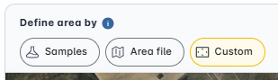
Once Custom mode is selected you can zoom in to an area and use the Boundary tool options to draw directly on the map or add a rectangle over your area of interest.

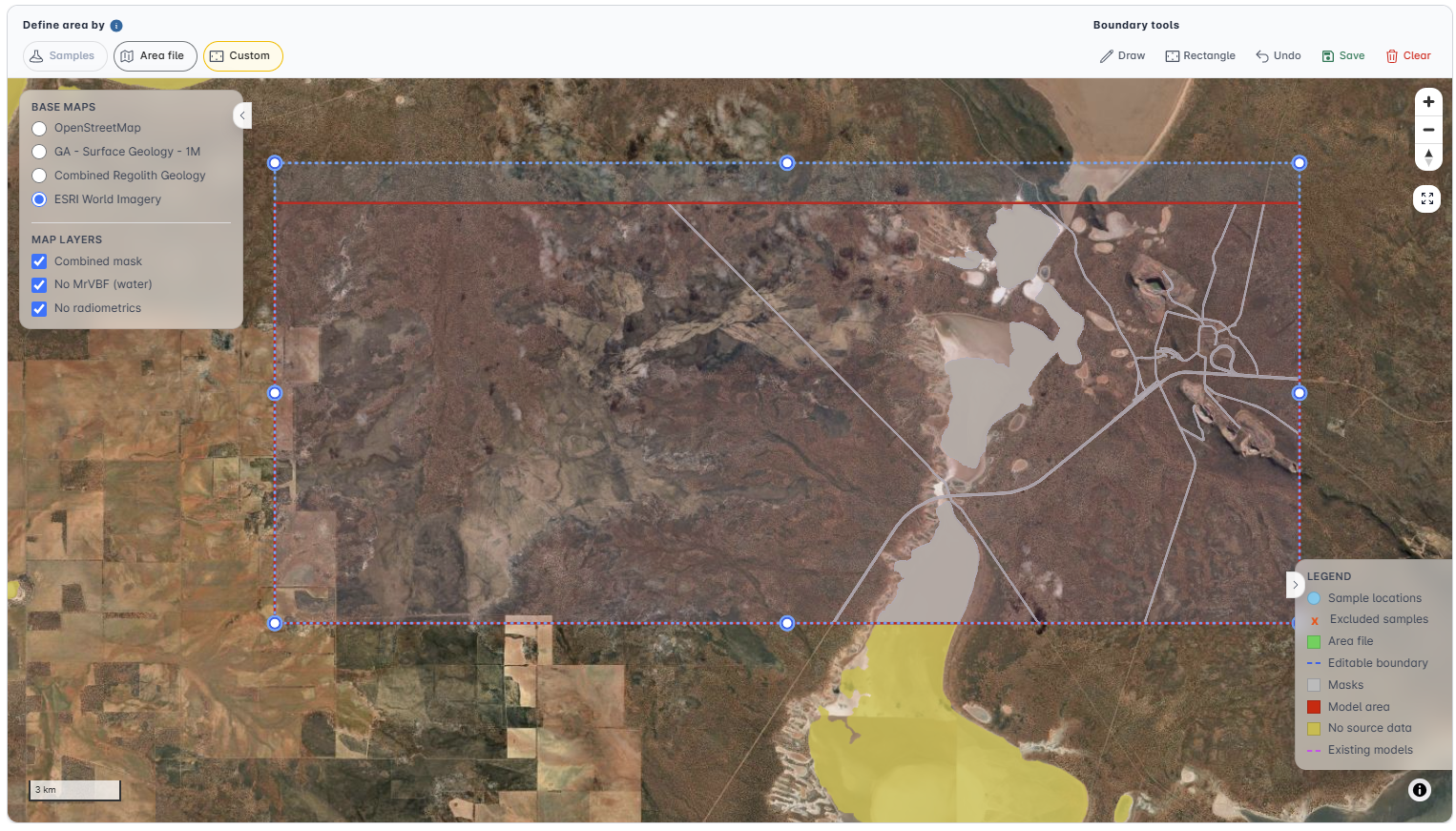
You can customise the extent of the model area further using the Editing tools in the Map viewer window and/or by double-clicking on the model boundary in the Editor window. The fill of the model area will turn transparent purple and white circles will appear in each corner of the model area outline box. See Resize model area in the next section for further details. The shape of the model area will always be a square box.
If you draw you can click multiple points to create a polygon. Once you double click the polygon will save to a rectangular shape that will be your model area, or you can click save. The option to draw a rectangular area is also similar. Note that areas that are masked automatically are shown in the map. These can be turned on and off to view, but it is critical to note that your model will never include these areas (e.g. water features).
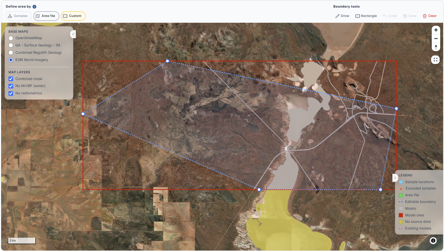
If the shape is not correct, simply click the Clear button and try again. You can also now use the features to adjust the red area rectangle by double clicking on the red outline. Once satisfied, click Save to continue. The legend in the lower right corner of the map explains the layers and gives clues to what is editable. The area of the model is displayed above and will be green if okay to proceed and red if it is not a valid area (too large or too small usually). Other information may also be displayed – see Map view window tools.
Adding samples to existing models OR adding a model to existing samples
In the side menu you can locate previous runs of models. Once selected, you can add a new geochemical data set to an older model. Click on the three horizontal lines next to the Project Title (“Demo 2026”) to see these features.
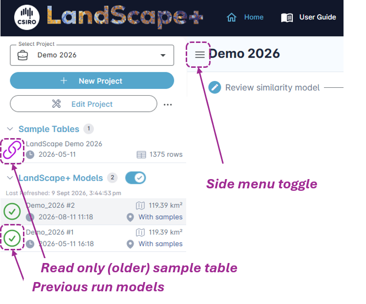
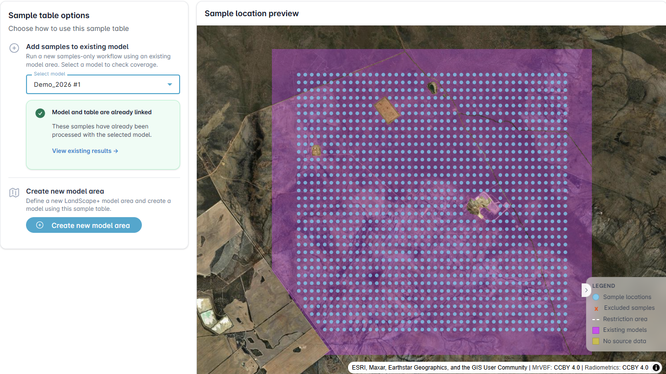
An option to add older geochemical sample tables to a newly created model is also facilitated here. Note that the linked purple icon indicates a data table data that is linked to an existing model (so cannot be modified or deleted). The table can be linked to additional models by selecting a model and clicking "Add samples to model". Alternatively, create a new model with this table by selecting "Add to new model".
The green tick shows models that are already run (with and without samples). Clicking these will load the model to which you can chose to add a new geochemical data set. You can toggle between samples that are included in the model under the “Review results” button in the Primary task stepper.
Opening an existing model will highlight that model area in purple shading on the map viewer interface. This will allow you to decide if you would prefer to adjust your model area. These sample tables can be selected in a new run and edited. A new sample table can also be uploaded. Help information opens when you click on each to guide you through the option. To add samples to an existing model, click on the model you wish to add samples to and then click “Add samples” in the Primary task stepper menu. From here you can create a new table or use the Select table drop down to add an existing data set to the model.
Once multiple models and multiple sample sets have been added to a project, you can toggle relatively quickly between geochemical data sets by selecting them from the Included samples drop down menu.

You cannot display two different geochemical data sets at the same time. You cannot display two different models at the same time. Loading an alternative model is slower than loading a different geochemical data set.
Note results for earlier versions of LandScape+ can be modified, however, there are limitations to the functionality and geochemical data may be better used if uploaded again as a “new” data set to ensure full functionality in the user interface.
By area file
You may choose to upload an area file such as a tenement boundary or other boundary you wish to use to define the outline of your model area instead of using the sample locations.
Click on the Area file button. A pop-up window will appear. Drag-drop or browse any area files you wish to upload. Note that the file has to be a GeoJSON, GeoPackage (.gpkg) or an ESRI Shapefile. If uploading an ESRI Shapefile, you must include all shapefile components (.shp, .shx, .dbf, and .prj files).
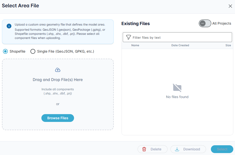
The Area file (dashed green polygon) will load into the Map viewer window and the Model area (red square) will update to fit around the uploaded shape. The Model area will always be a square. You can continue to use the Area buffer to change the extent of your Model area. It will now be centred around the Area file.
You can only display one area file at a time. If you wish to trial a different area, remove the current one, by clicking the small red cross in the Area file box (see image below).
You can revert the model area extent back to "Sample locations" by clicking on the corresponding button.

Map view window tools
The Map view window contains several functions to change the extent of your model area. A left mouse click will activate the Edit layer function. The area will turn semi-transparent red and Round handles will appear in the corners. Click and drag the handles to resize the box. Release the mouse to lock in the changes. This function can also be activated using the Boundary tools button in the Map viewer and editor window, or by clicking on the Custom boundary button.
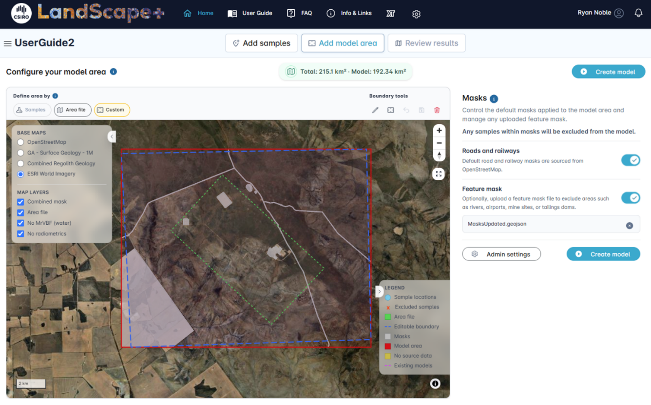
You may use the Pan function in the map window to drag your model area to a different location.
Note that any samples not within the model area will be excluded from the outlier definition and Principal Component Analysis. In such cases, an orange warning box will appear.
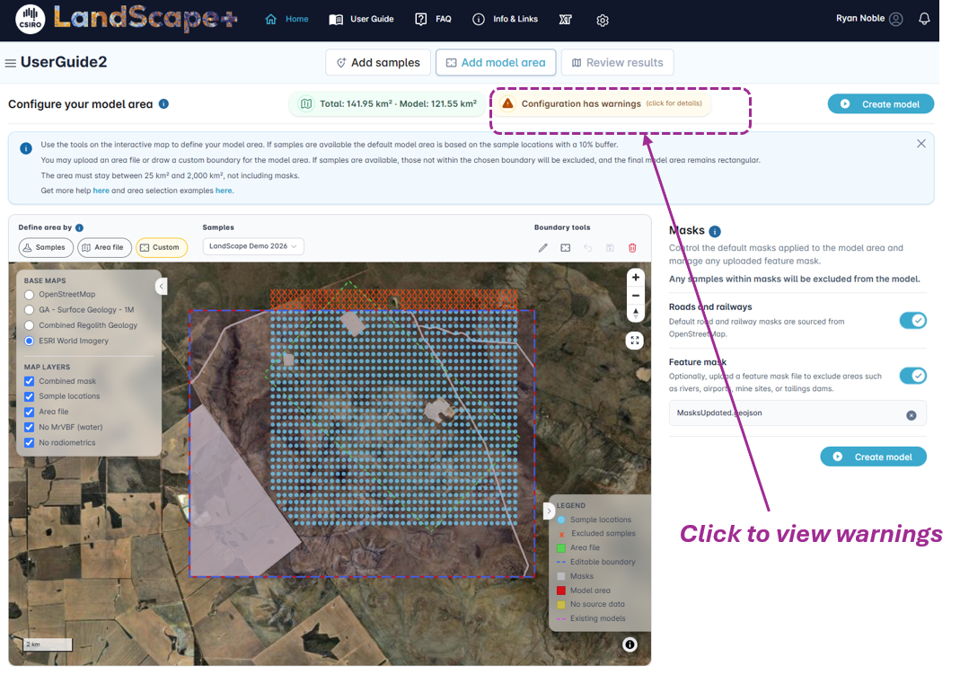
Click on the box to view details. Change the model area until you are satisfied that it captures the area you wish to model.
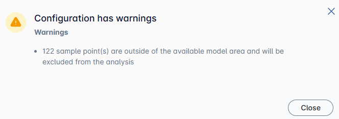
No matter the file or custom boundary you choose, the shape of the model will always be a square box.
When defining a model area, look for major features in the survey area you wish to capture and avoid small areas with few or no samples. For more guidance, see some examples below.
Select masks
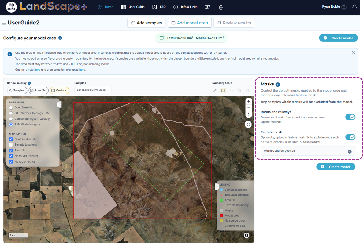
LandScape+® generates models from data collected at the surface which, with minor disturbance, is an expression of regolith and soil forming processes. However, the expression of these processes at the surface, and indeed the geochemical signature in samples collected in affected areas, can be disturbed by human activity. This includes major roads, railways, buildings and other infrastructure such as airports, mine sites, and tailings dams. We recommend masking such features in many cases.
Any samples that fall into masked areas will not be included in the model and no geochemical outliers or Principal Components will be calculated for those excluded samples.
All masks are displayed in grey and masked areas are automatically subtracted from the overall area size calculation.
No source data
The input, or source, data for LandScape+® includes radiometric data and MrVBF (Multi-resolution Valley Bottom Flatness index). The radiometric data of Australia does not cover 100% of the Australian continent and where this is missing, no model can be produced. The MrVBF excludes permanent water bodies (as per when the product was generated from SRTM DEM data; it may not reflect all current water bodies correctly), and such areas will also not be included in the model. This cannot be changed. However, most rivers and temporary water bodies are not excluded. The missing area of such source data is indicated in yellow in the Map viewer window.
Roads and railways
Default road and railway masks are provided and sourced from publicly available data (OpenStreetMap). Roads and railways are masked (i.e., the pixel that touches the road will not be included in the model) which is also generally a suitable approximate distance of sampling away from major roads due to the impact of contamination on soil samples.
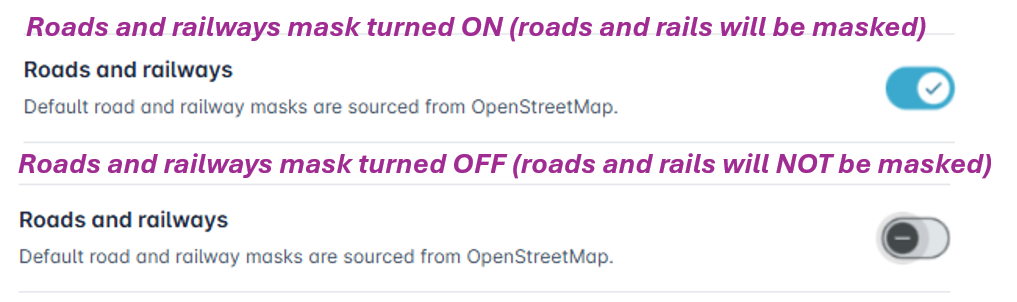
The Default setting is that this mask is ON (roads and railways will be masked from the model area and appear as empty lines).
We have provided the option to turn these masks off in case your soil survey follows roads or your model area is heavily traversed. If roads were present at the time of sampling and you have sampled along them, including them in the model will reflect the real-life context of your soil samples. Less frequented roads may have little effect on the model.
To remove the road and railways mask, move the Roads and railways slider to the left.
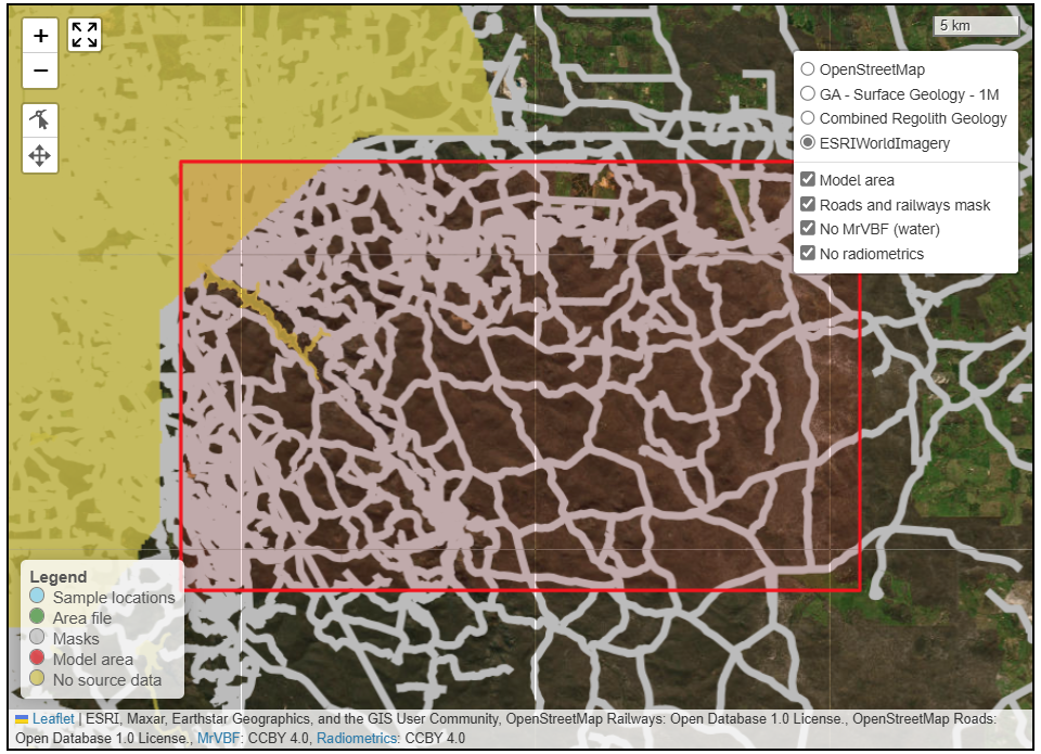
Example
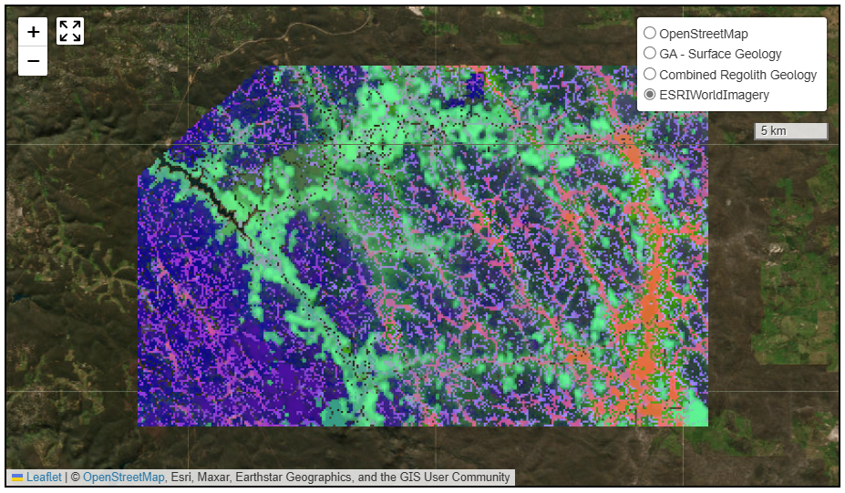
In the below example from the Mundaring state forest in Western Australia, the top left corner of the model area is masked out because no radiometric data is available. A permanent water body (the Mundaring Weir) is also masked out due to missing MrVBF data. An extensive network of roads and 4WD tracks has also been masked. Note that the masks are intentionally bolded in the user interface for visualisation – only the pixels touching roads are excluded.
The resulting model below has no infill for pixels in masked areas:
(continued from previous page)
Feature masks
You may choose to upload a custom Feature mask to exclude additional anthropogenic features, such as rivers, airports, mine sites, tailings dams, etc. from the model area. Mask data files can contain line or polygon geometries. All pixels that touch any mask geometry will be excluded. This is an optional feature and supported file types are GeoPackage (.gpkg), GeoJSON, or ESRI Shapefiles. If uploading an ESRI Shapefile, you must include all shapefile components (.shp, .shx, .dbf, and .prj files).
LandScape+ automatically saves your progress, so if you need to interrupt the workflow to draw a feature mask in a GIS software of your choice, you can close the software and return to where you left off at a later date.
Click on the Feature mask upload button in the Masks window. A pop-up window will appear. Drag-drop or browse any feature mask file you wish to upload.
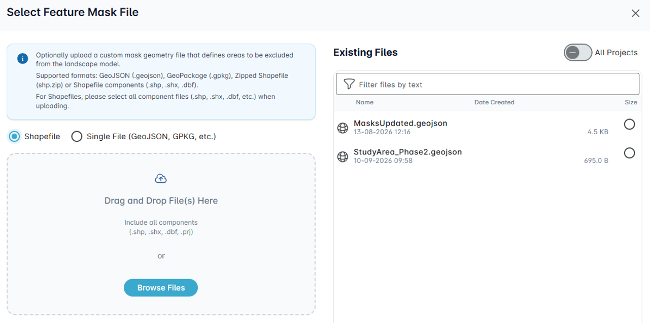
The Feature mask will display in the Map viewer and editor window in grey (same colour as the road and railways mask) and has been added to the Toggle menu.
You can only upload one feature mask file. If you wish to trial a different mask file, remove the current one, by clicking the small cross in the Feature mask box (see image below). You must use the Feature mask slider to include or exclude the masked areas from the model (see image below).
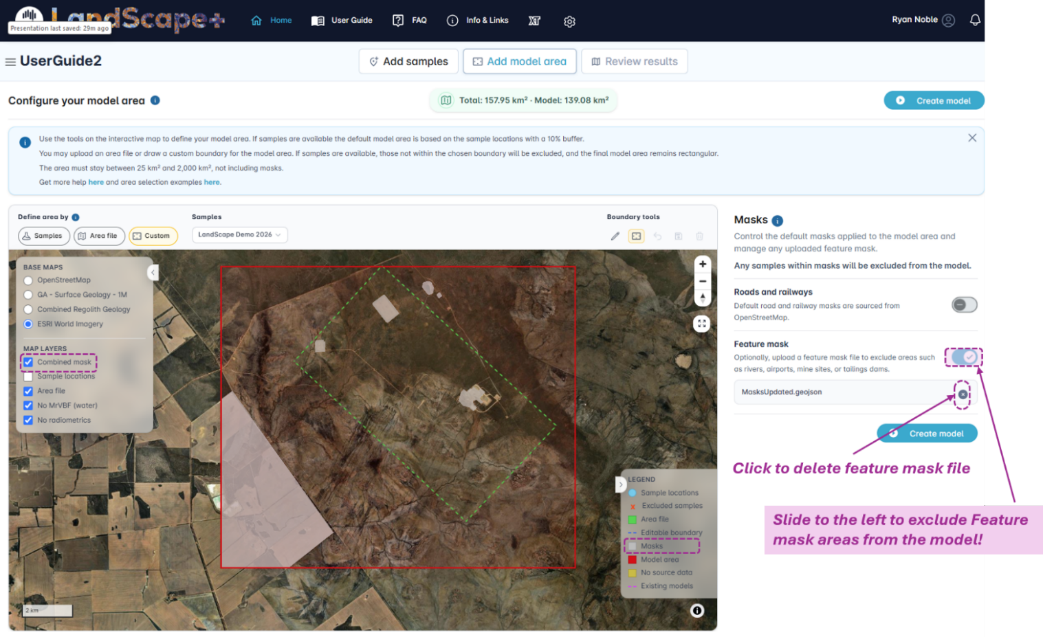
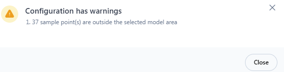
Once the mask is turned on, any samples that fall within masked areas will be excluded. An orange Warning box will appear.

Click on the orange Warning box to view details:
In this example, 37 samples fall within the masked area and will not be included in outlier definition. You can choose to remove, alter and re-upload the feature mask to include these samples bearing in mind that these samples may have been affected by anthropogenic disturbance. Or you can exclude these samples. There can be value in either option. In this specific example, soil samples were collected over mineralisation. A mine site was subsequently built and is part of the masked features.
It does not matter if your custom Feature mask overlaps with an in-built mask or an area of no source data. The model build process automatically combines all masks and areas with missing source data into one.