Principal Component Analysis

Your Data Package includes Principal Component Analysis (PCA) of all elements* for all samples* you uploaded with the aim to provide a first-pass multi-element geochemistry interpretation tool to identify potential areas of interest. Note PCA does not consider landscape types for the results, only the chemistry of the entire survey in the modelled area. Your data must have more elements than principal components (>5).

Overview

Principal Component Analysis is a statistical technique that reduces the variables (also called dimensions) of a geochemical dataset. All dimensions (elemental results) are transformed into a new coordinate system to describe the data with fewer dimensions (only five in this case) whilst preserving as much of the information (variation) in the dataset as possible. This makes the data easier to visualise and can be useful to identify patterns in a geochemical dataset using multi-element trends.

Disclaimer

Principal component analysis is a useful technique for first-pass identification of geochemical trends in a dataset with large numbers of variables and samples. A dataset with few analytes, few samples, or where a large proportion of data is at or below detection, may not necessarily be suitable for PCA and the user should be aware of this during interpretation of their results.

*PCA calculations

Principal Component Analysis is performed on centred-log-ratio and quantile-normalised transformed geochemical data for each sample. Each data point is reduced from n dimensions (number of analysed elements) into five principal components (PC1 to PC5). If more than 10 % of analyses for a given element are missing (e.g., as would be observed where the element has not been analysed) this element is not included in the PCA calculations. If less than 10 % of analyses of a given element are missing, the element is included in the PCA analysis, but no principal components are calculated for the affected sample that has that data missing.

PCA outputs

Spider diagram and spatial plots

LandScape+ produces a spider diagram and spatial plots as a PNG file. The spider diagram shows the loadings (weightings) of each element for each of the five principal components. This illustrates the general geochemical affinity of each principal component. The spatial distribution of each of the principal components by sample is also displayed in the PNG file below the spider diagram.

The spider diagram displays loadings for each principal component by a coloured diamond for each element. These are relative and show whether the principal component is positively or negatively associated with this element. All elements included in the PCA analysis are sorted alphabetically from left to right with visual guiding lines every 4 elements (in grey). The further a diamond plots away from the 0 line (dashed black line), the greater the loading for (influence on) the specific principal component.

The boxes below the spider diagram show the spatial distribution of each of the five principal components weighted by both colour and symbol size. The top five elemental loadings (the greatest influence on this principal component, whether positive or negative) for each principal component are indicated in the headings above these boxes. The colour red indicates a positive component weight (association); the colour blue indicates a negative component weight (association). The larger the symbols the stronger the association.

The explained variance of the principal components decreases from PC1 to PC5. Lower principal components will, therefore, often pick out large-scale lithological variation as the major component(s). Principal components with exploration potential commonly explain less variance in the data than the major elements related to geological influence. Hence, principal components that explain less variance (e.g. PC4 and 5) may represent relevant components in the context of mineral exploration. In some cases, signatures relating to mineralisation will constitute relatively low proportions of variance and thus will not be represented by principal components.

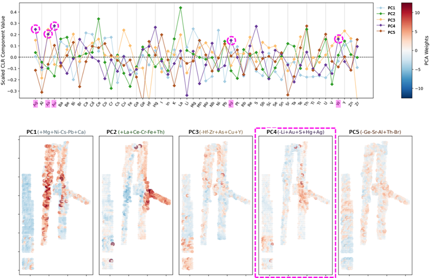
Example - Spider diagram and spatial distribution plots of principal components

In the below an interesting principal component for potential mineral exploration targeting with relatively high, positive loadings for Ag, As, Au, Pd and W is indicated in pink circles and shading (PC4; purple diamonds connected by a purple line)

Principal component shapefile and CSV files

Principal components for each sample are available as a shapefile for use in GIS software and as a CSV file.

Eigenvalues (CSV file)

Eigenvalues indicate how much of the variance in the data is explained by each principal component, as a percentage for each principal component.

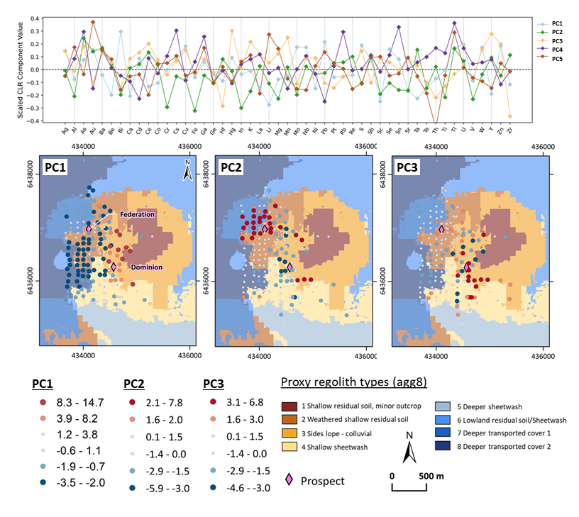
Example – Federation and Dominion Prospects

In the example below of the first three principal components from the Federation Project site (read the full report here), the first principal component (PC1) explains 46 % of the variability within the dataset and, unsurprisingly, highlights shallow geology and climatic influence (slope aspect or elevation) and matched the landscape proxy types/colours in the background. PC2 explains 18 % of the variability within the dataset and is associated with As, Au, Ta and Tl. PC3 only explains 15 % of the variability within the dataset, but also shows exploration potential with association of Ag, As, Cd, Cu, Hg, Ni, S, W and Zn. It therefore has positive loadings with some target and pathfinder elements such as Ag, Cu and Zn, but not with Au or Pb. PC3 also is strongly influenced by Mn in the samples. In retrospect, it appears that PC2 highlights the Federation mineralisation (downslope from and immediately to the northwest of the Federation prospect) and PC3 highlights the Dominion prospect (positive PC3 scores coincide broadly with the Dominion prospect and are positive; they are more subdued around Federation).