Step 4 – Review model outputs

Once your results are ready, you will receive an Automated email from no-reply@exploration.tools with a link to the Results page.

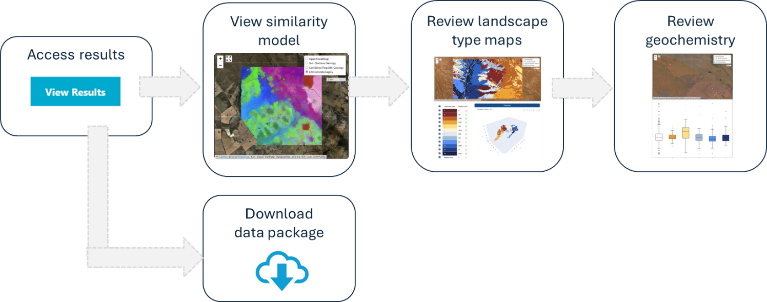
There are three main steps:

1. Review similarity model to familiarise yourself with what influences the landscape types in your model area

2. Review landscape maps with different amounts of landscape types

3. Review geochemistry and outliers by landscape type

We recommend that you review the results in the online User interface to decide which model is the best fit for your area. The interface will guide you through the decision-making process.

However, you can download all 12 landscape models as a Data Package at any time to use the outputs in a GIS software of your choice. Simply skip all model review steps in the user interface and go straight to download. The content of the Data Package download will not be affected by any actions you take in the user interface (except for the delete/remove entire project/results - which is not easy to do and has multiple warnings).

You can return to the user interface to review the model at any time for the duration of your licence (for one year after activation of the licence). Make sure you download the results before your licence expires.

4.1 Access results

Click on the Link in the Automated email or simply log into your LandScape+ account and click on your Project. When your model is completed, it will automatically open to the Results page.

The results include a similarity model and 12 landscape models for the same area. Each model includes a landscape map with different numbers of landscape types (4-16) and the landscape models include outliers by landscape type for each element based on each map.

Once you access the User interface, a pop-up dialogue box will appear with some important information. Read it while your model is loading in the background.

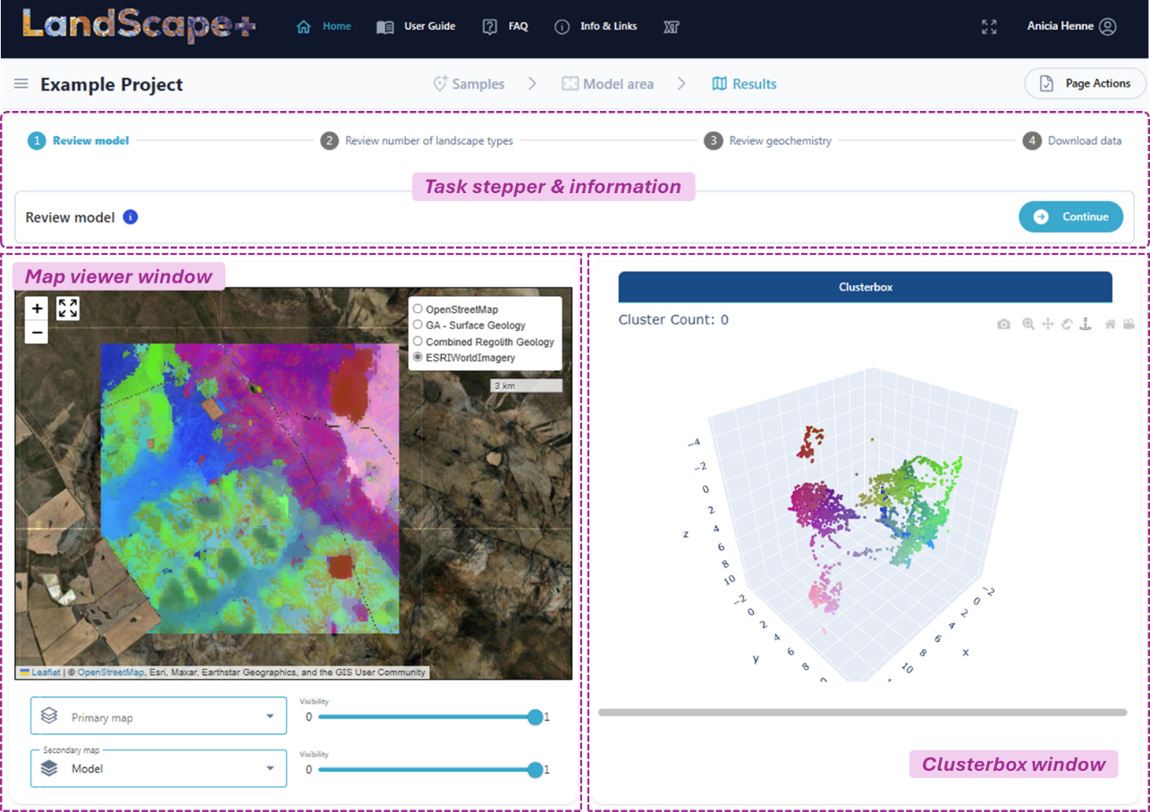
4.2 Review similarity model

The first content you will be able to view in the user interface is the similarity model (the landscape model coloured in RGB based on UMAP which is used to reduce the spatial dimensions – see Science Background box below if you want to know more). This is the basis for your model and you can view this in 2D in the Map viewer window and in 3D in the Clusterbox.

This output is not categorised, i.e., there is no hard boundary between pixels that would combine a group as one landscape type. This step is to familiarise yourself with the underlying spatial model before you view the landscape maps, and the User interface functionalities.

The Task stepper is accumulative so you can skip ahead at any time and also come back to this step later.

BACKGROUND

LandScape+ uses Uniform Manifold Approximation and Projection (UMAP), a dimensionality reduction algorithm, to transform the spatial input data for each project area to a three-dimensional representation of data. The method does not explicitly include any location information, spatial relationships, or spatial features (e.g., textures) as only the per-pixel values of each input layer are considered.

After UMAP has been applied to the input data, an agglomerative hierarchical clustering algorithm is used to group locations with similar data signatures. You can find more information on these algorithms here.

✔️ Compare input layers

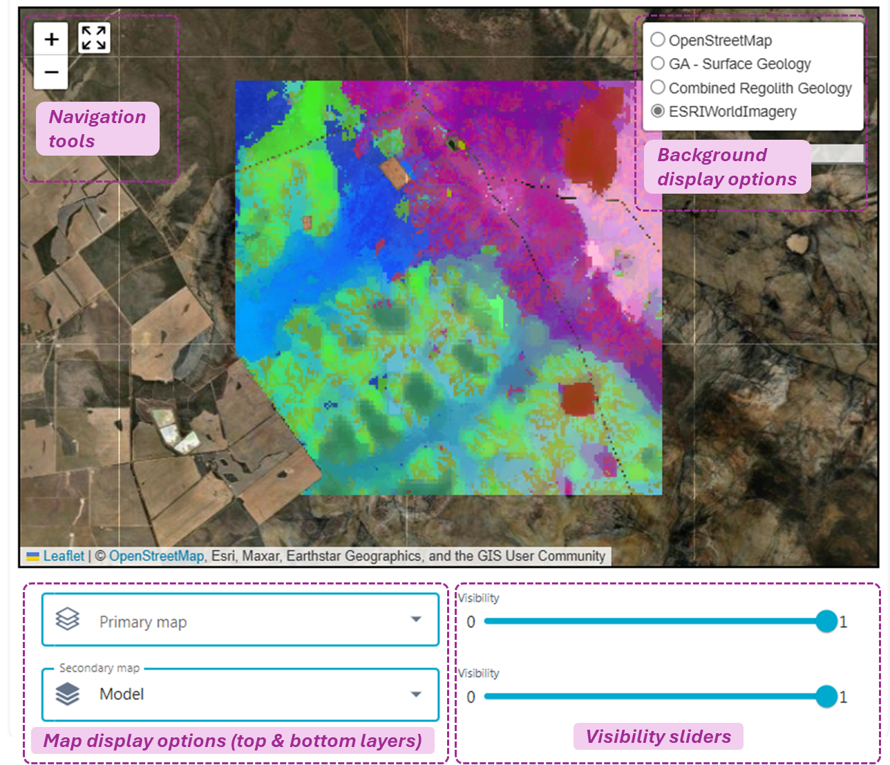
In the Map viewer window, select and compare the similarity model map to the different model input layers that have been used to create the model. Using the Map display options for the top and bottom layer, you can view two maps at the same time (e.g., the similarity model map and one input layer).

Select a layer in the Primary map drop-down and/or Secondary map drop-down. Options are the similarity model, Digital Elevation Model (DEM), Multi-resolution Valley Bottom Flatness (MrVBF), radiometric data, and Sentinel-2 ratios. You can choose either of these layers as both the Primary and Secondary map. Use the Visibility sliders to control the transparency of each map layer.

Use the Navigation tools, to Zoom in, Zoom out or return to the Model extent.

Change the Background display by using the Radio buttons in the Background display options. Available spatial layers are OpenStreetMap, Surface Geology, Combined regolith geology (a combination of GSWA and GA regolith geology layers) and Satellite imagery.

Example

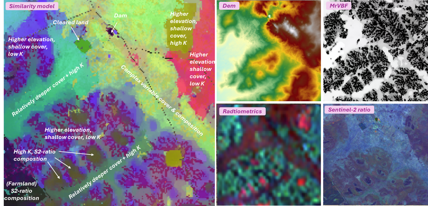
The below example without any masks, shows a rapid overview of the main input features that influence the model. Identifying the main features, will help you decide how many landscape types you might want to choose in the next step.

Tip

Place the model at the top (Primary map) and the input layers at the bottom (Secondary map), then use the Visibility sliders to fade the model in and out to see which features are influenced by which input layer.

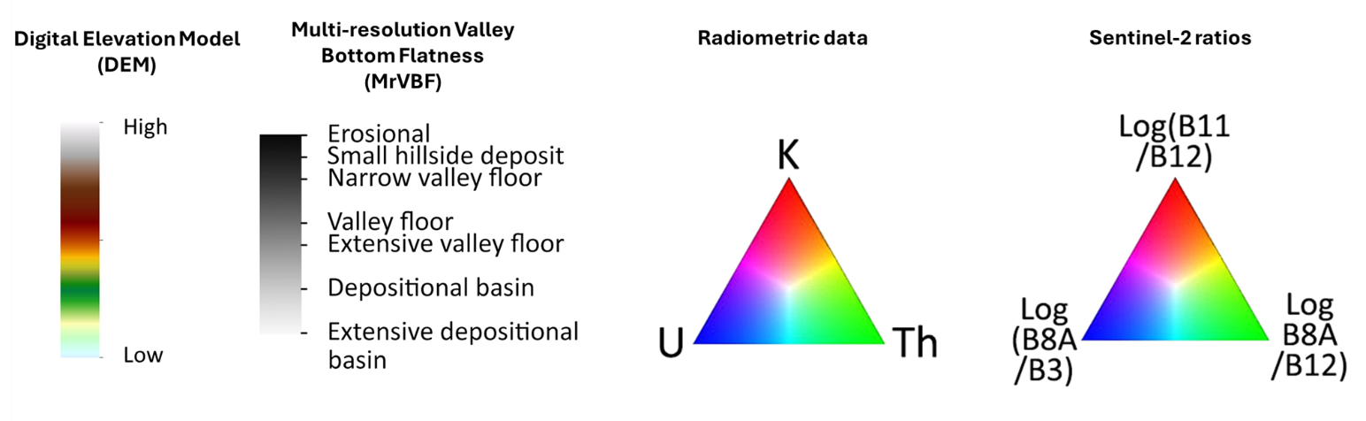
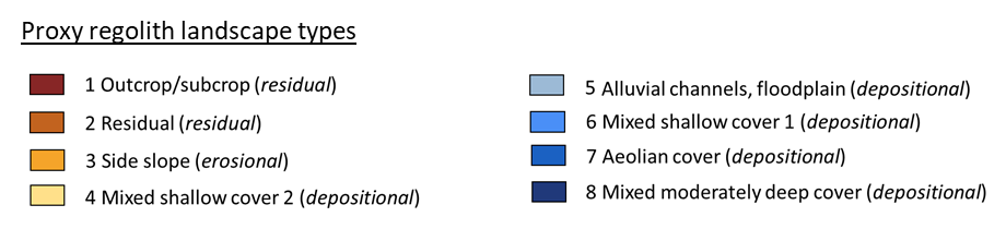
Input layer display legends

✔️ Review Clusterbox

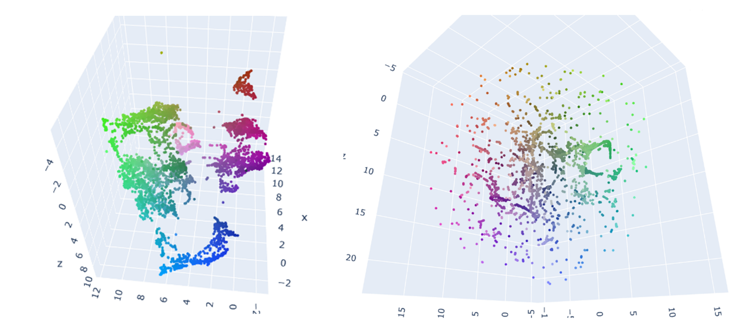
The Clusterbox is a 3D representation of the pixels on the map. The closer pixels are clustered together the more similar their modelled input layer attributes. If most points are equally close together (forming a uniform “cluster” or “cloud”) there is likely not much landscape variability in the modelled area. Similarly, if you have a dispersed “cloud” of pixels that do not form “clusters”, this also indicates little landscape variation. Points that form distinct clusters, especially offset from other point “clouds” indicate that you have distinct landscape types.

Click and hold your mouse over the Clusterbox to rotate and view each cluster in more detail. You can also Zoom in and out. The colour of each pixel in the Clusterbox is the same as its colour on the map.

Example of a useful and a less useful model (Clusterbox)

A useful model displays multiple distinct clusters (left) and indicates distinct landscape types with different properties. A less useful model will display no or few distinct clusters and/or a fuzzy cloud of individual pixels (right) indicating little landscape variation within the chosen model area, or variation that cannot be captured with the model input layers. If this is the case for your model, you may modify your model area to capture greater landscape variation in your next model run.

✔️ Continue

Once you have familiarised yourself with the model, click on the Continue button or click on Select number of landscape types in the Task stepper to proceed.

4.3 Review landscape type maps

The User interface will now have two additional functionalities. The Landscape type number menu underneath the Task stepper at the top of your screen and the Samples overview table.

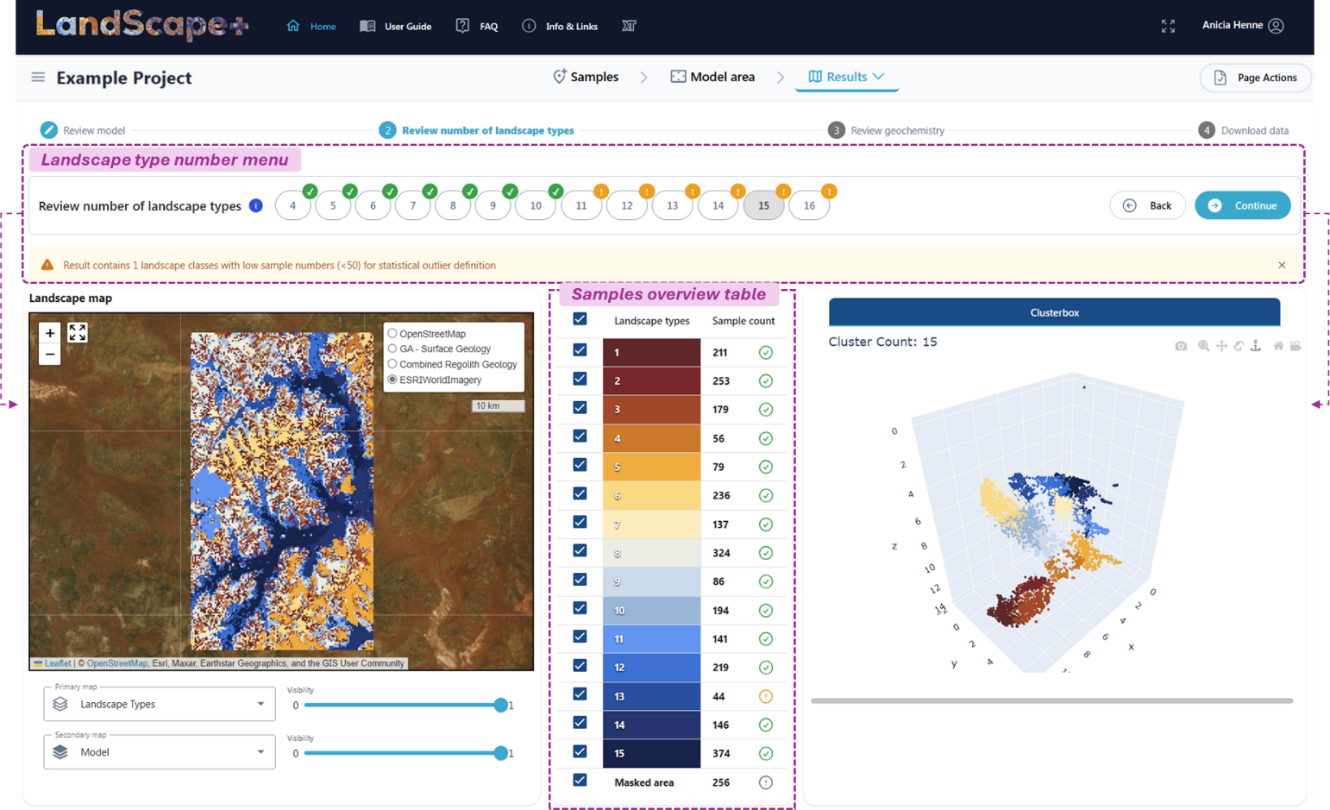
The Landscape type number menu contains 16 Landscape number buttons. The number on each button corresponds to the number of landscape types in the map, i.e., clicking on the button with the number 4 will show you a landscape map with four landscape types. Clicking on one of the buttons will update all content on the page. - Both the pixels in the Map viewer window and in the Clusterbox will be coloured by the number of landscape types you choose with the Landscape number buttons.

✔️ Review maps and clusterboxes

Review the available number of landscape types by toggling between the Landscape number buttons. The map in the Map viewer window and the colours of the pixels in the Clusterbox will change accordingly. Ideally each colour represents a distinct cluster of pixels in the Clusterbox and a distinct landscape type on the map in the Map viewer window.

The model forces pixels into separate groups to satisfy the amount of landscape types you choose. The highest number of landscape types therefore does not always produce the best model.

You will already be familiar with your model from the last step and will have an idea of how many different landscape types you would like to see in your map. The best Landscape type map will resemble the similarity model.

✔️ Compare landscape maps to other spatial layers

Once you have narrowed down how many landscape types best fit your survey area, select Model input layers (the Digital Elevation Model (DEM), Multi-resolution Valley Bottom Flatness (MrVBF), radiometric data, and Sentinel-2 ratios) in the Map display options from the Primary map drop-down and/or Secondary map drop-down to compare to the different Landscape type maps just like in the previous step. Use the Visibility sliders to control the transparency of each map layer and use the Navigation tools, to Zoom in, Zoom out or return to the Model extent.

Make use of available surface and regolith geology maps by changing the Background display in the Map viewer window using the Radio buttons in the Background display options. These can be helpful in some settings.

Example

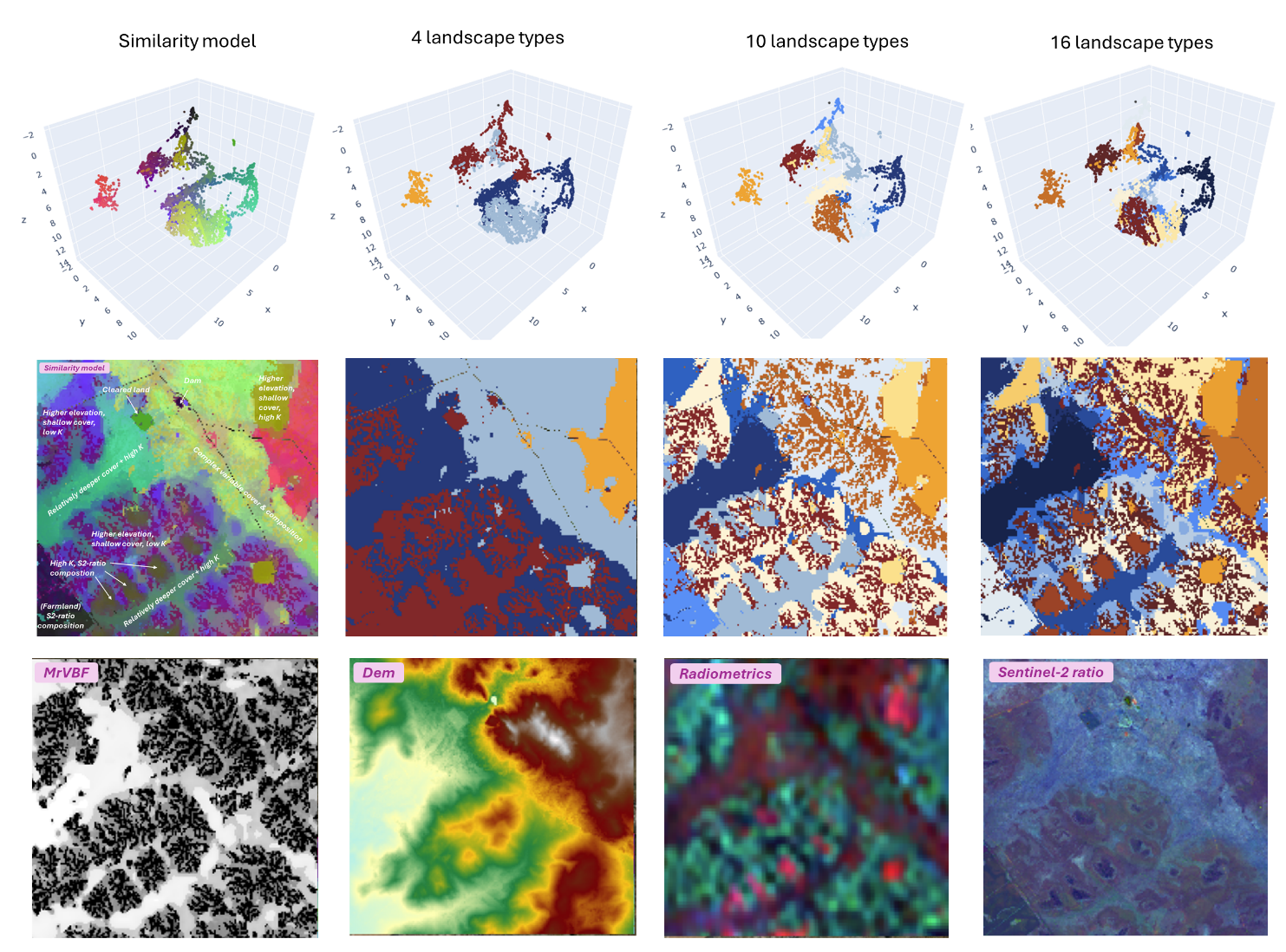
In the example below the Similarity model shows several distinct clusters of pixels. These are reflected in the 2D map. The map with four landscape types draws out deeper cover in dark blue, areas of shallow cover in dark red-brown, areas of higher elevation in light blue, and the low K radiometric signature in the NW (orange), but it does not represent other features identified in the last step. The map with 10 landscape classes has added more detail (e.g., farmland in mid blue in the SW) and a radiometric K high in the NE (light yellow). If, for example we were interested in picking out the other radiometric anomalies in the south-west as a separate landscape type, these are present in the landscape map with 16 clusters. However, this model divides the clusterbox pixels into groups that are hard to separate visually and adds potentially unnecessary complexity to the map. If the radiometric K highs are important, the ideal output would be more than 10 and less than 16 landscape types. Quickly toggling between the different landscape numbers has narrowed down the options sufficiently to move on to the next step (reviewing the number of samples per landscape type).

Tip

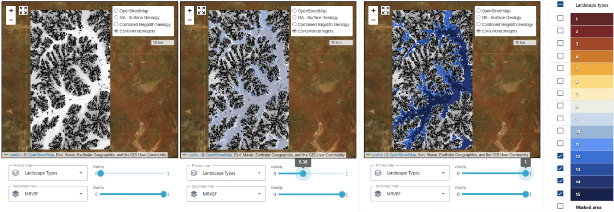
You can show/hide different landscape types by ticking/unticking the boxes to the left of each landscape type in the Sample overview table. This can be very helpful to interpret the different landscape features that the mapped units represent. In the example below only dark blue landscape types are displayed.

By displaying the MrVBF in the Secondary map (bottom) and the landscape types in the Primary map (top), it becomes obvious that these landscape types are in depositional settings of deeper cover. An appropriate descriptor might be Channel materials with lighter blue shades at higher elevations and more shallow cover. Overlaying these over the other input layers may enable more thorough definitions on their relative composition or radiometric signature.

A note on landscape map colours

In general, all landscape types are ordered by cover thickness (MrVBF) from dark red-brown to dark blue.

The MrVBF scale is relative (based on the lowest and highest mean MrVBF values in your area), and low values indicate shallow depth of cover, whilst high values indicate deeper cover. The lowest mean MrVBF values in your model are assigned a dark red-brown colour, and commonly indicate outcrop/subcrop/residual cover grading into orange/yellows/light blues for side-slopes, channel deposits, shallow cover. The highest mean MrVBF values in your model are assigned dark blue and often indicate areas of deep transported cover. The darker the blue the deeper the cover usually is on a relative scale within your model area.

However, since the MrVBF is relative, occasionally, the presence of elevated lowlands (e.g., depressions in higher elevation regions of your survey) or outcrops in otherwise deep cover (e.g., silcrete outcrops on salt lakes) can influence the order of landscape colours you might expect. The colours based on MrVBF provides a useful visual ranking but does not indicate the magnitude (or form) of differences between landscape types. Especially for models with higher numbers of landscape types, it is common to have multiple landscape types with similar mean MrVBF values which differ in other properties.

Each site is processed individually, and landscape types cannot be compared to other sites. What is yellow at a study site in the Pilbara is not at all comparable to what is yellow at a study site in the Yilgarn, or even on the adjacent tenement package if it was processed separately.

Background

The process of clustering data into proxy landscape types inherently puts a hard boundary on the data (the computer is forced to make a decision) even though, in many cases, there is a gradual change and the exact location of the boundaries is somewhat arbitrary. This is no different to other geological maps, although less biased than human interpretation, and analysis of samples near cluster boundaries should be considered with caution.

MrVBF - A key difference to traditional regolith maps

A key difference between the machine learning derived landscape type maps and a more typical regolith surface map is the inclusion of the MrVBF layer. For surface exploration it is essential to evaluate anomalies distinctly based on the thickness of cover and the MrVBF provides an estimate of this feature. Some areas might look different to traditional regolith maps because of this. This can be particularly pronounced for alluvial channels which might switch colours on the maps. This is because the overall landscape cover thickness has changed with the MrVBF. Hence, although the samples may be in a similar geomorphological setting (fluvial channel) the depth of cover has changed. This is important information in the context of surface geochemistry, since the elemental signatures in deeper cover are likely to be weaker or perhaps unlikely to be detected with surface geochemical techniques. This enables better discrimination and consideration of the geochemical data. A similar observation occurs in sheetwash plains and sand plains as the landscape proxies extend across paleochannels. On the surface, they may look similar, at depth there might be a lot of change with potential paleochannel features and this is not generally captured in a traditional regolith or surface geology maps.

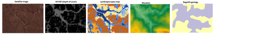
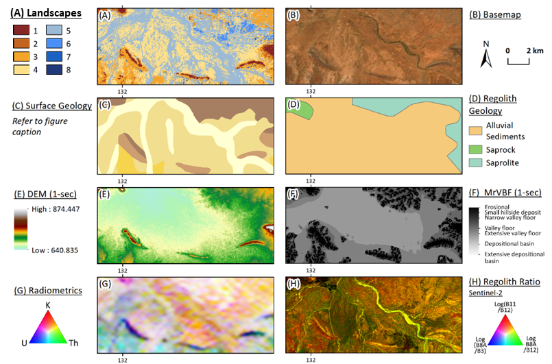
Example - Similar regolith material with changing depth of cover

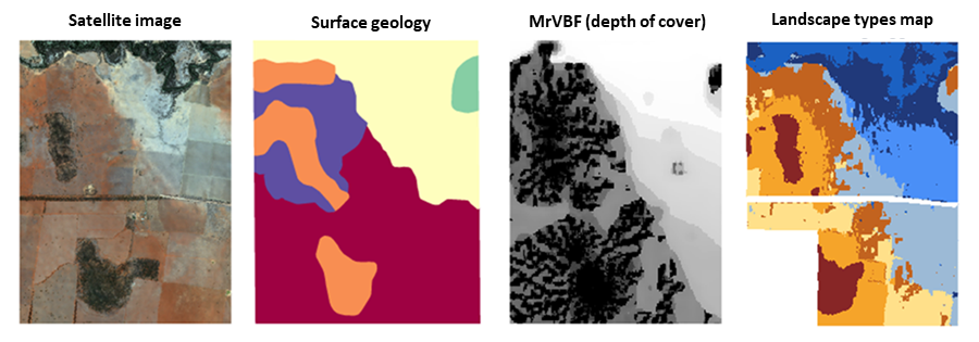
In the below example, the satellite image shows a river on the northern (top) edge. The mapped surface geology notes the yellow unit as an alluvial plain and the dark red-brown unit as a sand plain. The MrVBF shows changing depth of cover (from relatively shallow in the south to relatively deeper in the north) that are not reflected in the surface geology. However, in the landscape model the alluvial plain is broken into three shades of blue and the sandplain into three landscape types of pale yellow, brown and grey blue. These six landscape types show the gradual thickening of the cover as both the sandplain and the alluvial plain stretch away from the upland regions. From a geomorphological perspective, the surface geology provides valuable information, from a 3D exploration perspective it does not include key information for the surface explorer.

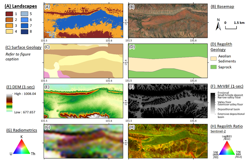
Example 2 - Alluvial channels with different colours

The example below shows drainage channels in an upland setting of ≈ 2km². Whilst the general drainage area is evident in the satellite image and in a more general but broader sense in the elevation and regolith geology maps, the landscape type map shows the drainage channel as mid blue and dark blue. On the surface this region is similar, but the MrVBF shows the broader, flatter depositional nature in the channel, which triggered the model to separate the channel into two landscape proxies.

✔️ Review the numbers of samples in each landscape type

The Sample overview table provides a summary of how many samples fall within each landscape type and will also update by clicking the Landscape number buttons. This number will change with changing amounts of landscape types depending on sample locations. The green ticks and yellow, red or grey exclamation mark Icons in the Sample overview table relate to the robustness of outliers that are calculated for each element in each landscape type. We recommend a minimum of 50 samples in each landscape type for meaningful statistical outlier definition. The Icons give some guidance to allow you to make informed decisions. A landscape model with less landscape types than is ideal for your project area might be preferable because the main aim of the LandScape+ outputs is to provide context for your geochemistry.

The Yellow information box below the Landscape number buttons provides a summary of what to look out for.

Selecting an appropriate number of landscape types is a balance between representing the major landscape types in your area whilst also enabling meaningful interpretation of geochemical data.

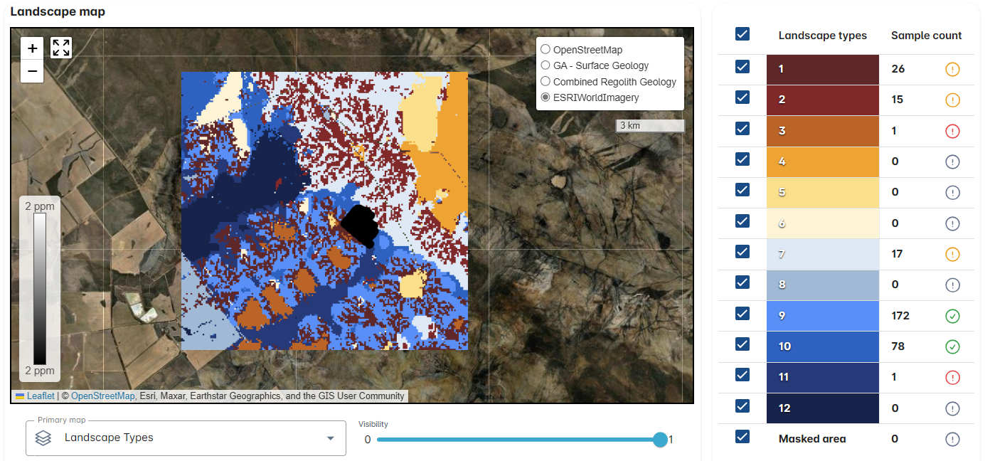
Example – Landscape variation vs. number of samples

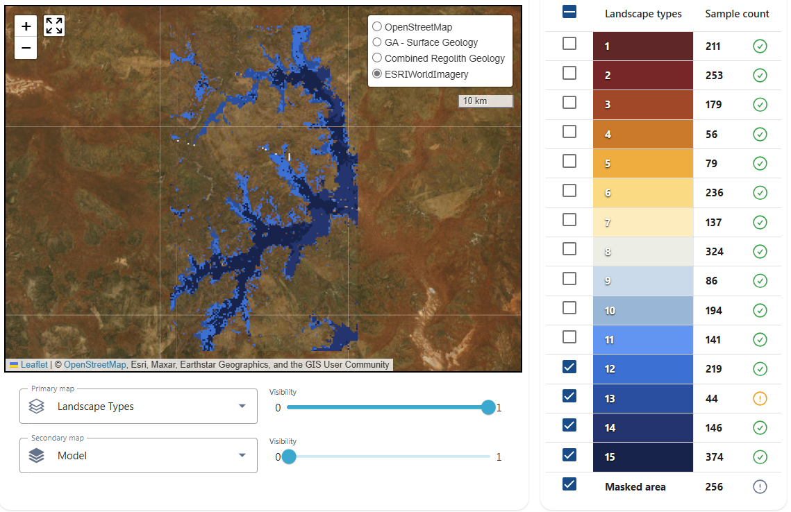
The example below has been purpose run using fake geochemistry to illustrate the issue of running a large model area for a small, concentrated survey of less than 300 samples. When the map with the ideal number of landscape types is chosen, only landscape types 9 and 10 contain sufficient samples. Whilst the map can be very useful to plan extension soil surveys, it is less useful for outlier definition.

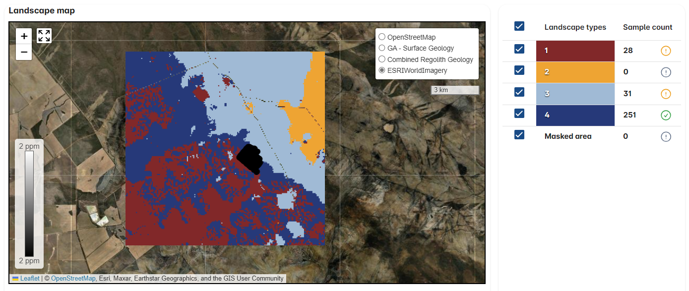
Even the map with 4 Landscape types allows only for review of the geochemistry in landscape type 4 with high confidence, and landscape type outputs 1 and 3 have been flagged as containing low samples. Whilst it is prudent to review these samples as a whole population in addition to grouping them by landscape type, the map does provide landscape context – landscape type 4 (dark blue) is a depositional regime with relatively deep cover, whilst landscape types 1 and 3 are distinguished by higher elevation. As such, samples in these settings are up-slope whilst samples in landscape type 4 are downslope – the model still provides context for interpretation of the results.

✔️ Naming your landscape types

The model identifies patterns and structures within the input data independent from human input such as regolith or surface geology maps. This means that the resulting map units are not labelled and have no description.

There are no naming conventions, and you do not have to give your landscape types a name, but you generally need to know whether you are looking at depositional, residual or erosional landscapes and review the MrVBF layer in the Map viewer window to identify whether the landscape types represent none, some, moderate or thick cover. Some landscape types may be a mix such as residual soils trending into colluvial soils (erosional side slopes).

Put general notes or terms against the colours to help fine-tune your understanding of what the colours commonly represent. You and your exploration team will know your area, and it is likely that you will associate certain landscape settings with a distinct colour of the modelled landscape types.

Use the Navigation tools in the Map window viewer to Zoom in on clearly identifiable features and look for similarities that will explain why these data are grouped.

For example, Zoom in on areas with outcrops or residual hills (note the colour) and look for these features elsewhere. Is it the same colour? Commonly, you will start to recognise the same colours corresponding to similar landform features. Some obvious landscape settings to observe are active fluvial channels, river terraces, deltas and large linear dune fields. Some features may be less clear – erosional mid slopes trending into foot slopes, toe slopes, and pediplains/sheetwash plains can overlap in the different landscape proxies.

Example workflow for naming landscape types

It is likely that most landscape types identify landforms/regolith materials that you are already familiar with, such as outcrops or drainage channels. You know your survey area - utilise any other high-resolution data and your on-the-ground observations by downloading the Data Package and dragging a GeoTIFF (.tif) of your Landscape types map into a GIS software.

Whilst the below examples illustrate working in GIS software for ease of summary figures, you can complete the same reviews in the User interface in a more interactive fashion.

Example 1 - Naming landscape types

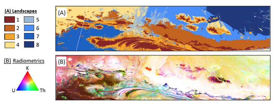
In the below example from the MacDonnell Ranges in the Northern Territory, those familiar with the general area will readily identify the dark red-brown and light brown landscape types in (A) as elevated ranges, and the radiometric data (B) points to differences in parent material between the two. An appropriate ‘name’ for these landscape types may be outcrop/subcrop (dark red-brown, 1) and residual (light brown, 2) landscapes.

Zoom in on prominent features, such as outcrops, to label further landscape types:

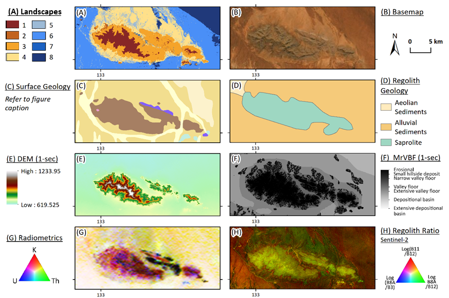
The satellite image (B) shows a pronounced outcrop, the DEM (E) and MrVBF (F) indicate differences in landscape position and depth of cover between dark red-brown (1) and orange (3). An appropriate ‘name’ for landscape type 3 (orange) may be side slope. Further downslope (light yellow, 4, and blue colours, 6 and 8), the Sentinel-2 ratio map (H) indicates a change in regolith materials, which is strengthened by a change in the radiometric signal (G) as well as the depth of cover (F). Both, light yellow (4) and mid blue (6), are mixed shallow cover, which may be termed shallow cover 1 and shallow cover 2; the main distinction being the difference in depth of cover. The dark blue landscape type (8) represents the relatively deepest cover and may be termed deeper cover.

Zoom in on other prominent features such as channels, to label further landscape types:

The light grey-blue landscape type (5) is in a generally low landscape position (E) with deeper cover (F) and the Sentinel-2 ratios (H) show different regolith materials which match distinct river channels in the satellite image (B). We may ‘name’ this landscape type alluvial channels and/or floodplains, and the spatial association of this landscape type with surrounding colours also provides more information about the pale yellow landscape type (mixed shallow cover 2).

Zoom in on the remaining unnamed mid blue landscape type (7):

The mid blue landscape type (7) is wedged between side slope material (orange) shedding from outcrops/subcrops (dark red-brown) to the north and south. The setting is a relatively lower landscape position (E) with deeper cover (F) and a distinct colour difference in the Sentinel-2 ratios (H; indicating a change in regolith materials). The satellite imagery identifies a sand dune. Through confirming these same features in other parts of the model area, we may name this landscape type aeolian cover.

The below interpretation provides sufficient context for geochemical outliers which have been calculated for each landscape type.

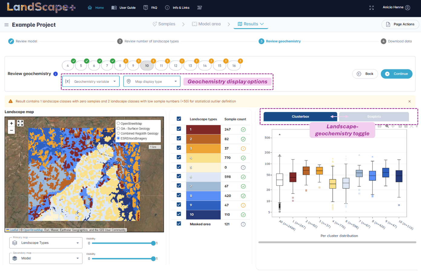
4.4 Review Geochemistry

The User interface will now have two additional functionalities. The Geochemistry display options underneath the Landscape number buttons at the top of your screen and the Landscape-geochemistry toggle. The Geochemistry display options allow you to view soil samples by geochemistry in the Map viewer window. The Landscape-geochemistry toggle allows you to toggle between Boxplots for each element and the Clusterbox for the model The Boxplots will automatically display once you choose an analyte in the Geochemistry display options.

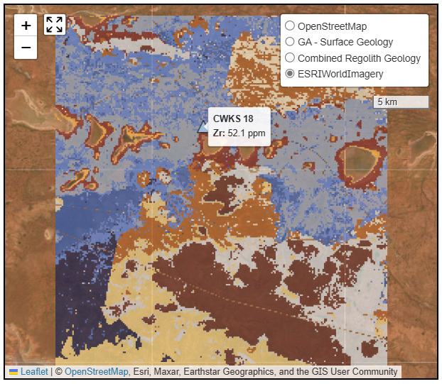
Tip

Hover over your outliers in the boxplots or on the map to display the Sample ID and concentration of your chosen analyte.

✔️ Review analytes and boxplots

Choose from the available analytes in the Geochemistry variables drop-down to display the analyte of your choice. The Boxplot will automatically populate and replace the Clusterbox. Samples will only appear on the map once you choose a Map display type from the Map display types drop-down.

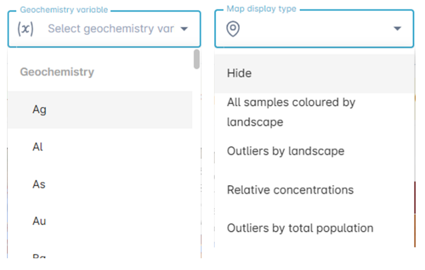
The following Map display types are available:

Map display type	Description
All samples coloured by landscape type	Displays all samples as coloured circles and outliers of the analyte chosen from the Geochemistry variables as triangles
Outliers by landscape type	Displays only the outliers of the analyte chosen from the Geochemistry variables as triangles
Relative concentrations	Displays all samples as circles in a grey scale from lowest to highest concentrations of the analyte chosen from the Geochemistry variables, outliers calculated from the entire survey data (not by landscape type) will display as triangles
Outliers by total population	Displays only outliers calculated from the entire survey data (not by landscape type) as triangles
Hide	Hides all samples from the Map viewer window

How to read Boxplots

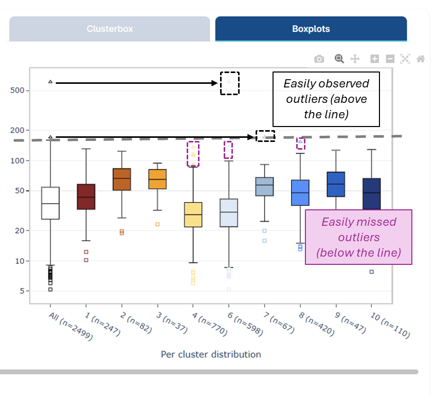
The Boxplots are Tukey plots and show outliers by sample population. They are linked to the Geochemistry variable drop-down, i.e., when you display Au on the map, the boxplot will also change to Au. Boxplots display outliers by total population (white box on the left-hand side) and outliers for each landscape type (coloured boxes). Outliers are indicated as triangles in the boxplots and on the map. Outliers may differ depending on the number of landscape types you choose.

The triangles above the white box are always the highest overall relative concentrations of the chosen analyte (1.5 times the interquartile range above the 3^(rd) quartile of the whole population). Outliers calculated for sub-populations in each landscape type are also the highest concentrations in their specific landscape type. However, they may be significantly lower overall. If we draw a line at the 1.5 times interquartile range (the dashed line extending from the top whisker of the white box in the figure below) this becomes more evident. Such outliers, below the line (see triangles in the dashed purple box in the figure below), would be easily overlooked or not identified without landscape context.

Example – comparison between total outliers and outliers by landscape type

In the example below, when outliers for zinc are calculated on the whole dataset, only two values display as outliers in the map and above the white boxplot (see white triangles in both the map and boxplot). When the same data is separated into 10 landscape types and outliers are calculated for each, more outliers are identified (see coloured triangles in both the Map viewer window and the Boxplots). This extends a potential area of interest in the south providing more confidence in this elevated concentration.

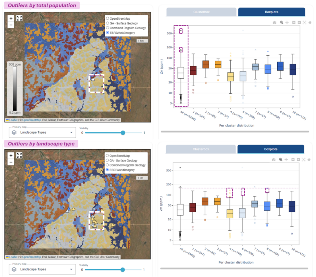
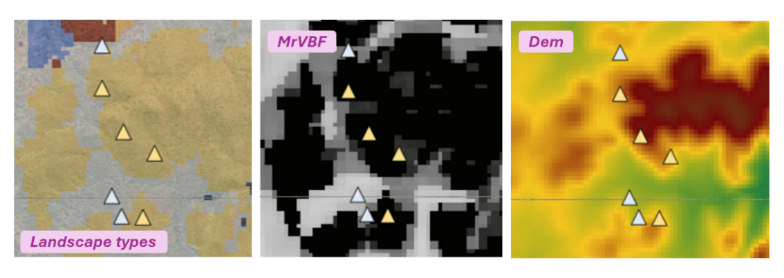
The User interface allows us to Zoom in on these outliers. Outliers are located in two landscape types. By toggling different input layer features we can easily identify that the light-yellow landscape type is in residual cover at relatively higher elevations, whilst the grey-blue landscape type is in lower landscape positions and likely deeper cover. It is reasonable to interpret the light blue materials to be channel materials which are potentially shedding from the residual settings upslope.

Critically low sample populations

When sample populations contain critically low amounts of samples (less than 15), statistical outlier definition may not be robust and such outliers must be treated with extreme caution. This is indicated by a Red exclamation mark icon in the Sample number overview table. Such outliers will display as Upside-down triangles in the Boxplots and in the Map viewer window with a smaller font size.

Yellow exclamation mark icons indicate low numbers of samples and these should be reviewed with caution.

Even if you don’t have the recommended number of samples for statistical outlier definition (50 or more) in a given landscape type in your favourite landscape model, you can compare outliers across multiple Landscape maps with different numbers of landscapes. If outliers remain outliers across different landscape types, this should provide more confidence that this outlier presents an unusually greater concentration of the chosen analyte than expected for this setting.

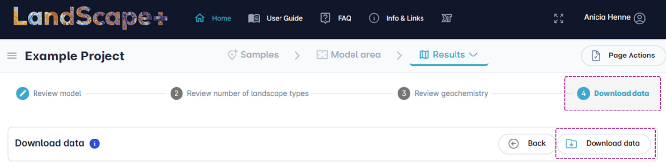
4.5 Download results

Depending on your area size and number of samples, your data package may be large (multiple GB), so ensure you have enough space on your disk and a good internet connection for the download.

Click on the Download data button to download your data. This will download all landscape models (12 models with 4-16 landscape types) and their corresponding outliers. This is your ‘hard copy’. You can return to the online User interface for the remainder of your licence (for one year after licence activation).

In addition to the online User interface, you will be able to view Principal Component Analysis results in your data package.