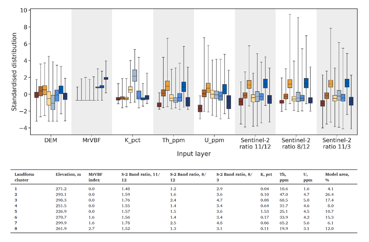
Distribution of spatial features
Each folder in the “Landscape type maps and outliers” of your Data Package contains a folder called Distribution of spatial features with additional summary outputs that may be useful for in-depth interpretation. The folder contains a Table with median pixel values of the spatial data features (input layers) for each landscape type and a visual representation of the distribution of all spatial data feature values by landscape type as Boxplots. The distributions in the boxplots are standardised per-feature (to a median value of zero and standard deviation of one) to visualise relative differences and similarities between features. This can help you identify how your landscape types differ. Although the Similarity model map and Clusterbox are a better 'overall summary', these additional outputs point to features that influence the differences and similarities in the landscape types. The Boxplots also provide an indication of the variation within your landscape types.
Example - Visual influence/weighting of model input layers
In the example below, the grey-blue landscape type, relative to other landscape types, is low in elevation, very low in MrVBF (likely residual to outcropping), shows high K composition, low Th and U composition and median Sentinel-2 ratios. This particular landscape type represents granite outcrops and very shallow residual soils over outcrops. The royal blue and orange landscape types have very similar pixel value distributions and median values in all input layer attributes except for the MrVBF index which indicates that the royal blue landscape type has a higher relative depth of cover index. These landscape types represent residual, ferruginous materials (orange) cut by river channels (royal blue) carrying eroded materials. To gain further insight and understanding on how to use this output, you can read more about the below example in this open access publication.